
Project finance modeling for renewable energy transforms solar projects from promising concepts into bankable investments by building a detailed, multiyear financial forecast that quantifies returns, manages risk, and demonstrates viability to lenders and equity partners. At its core, the process structures capital flows, revenue streams from power purchase agreements or merchant sales, operating costs, and tax benefits into a dynamic model that proves the project can generate sufficient cash flow to service debt and deliver targeted returns. Mastering this discipline is essential for project developers and finance professionals who need to secure the millions required to bring utility-scale solar installations from permitting through commercial operation.
The complexity lies in integrating diverse financing mechanisms. Modern renewable projects rarely rely on a single capital source. Instead, they blend tax equity structures that monetize investment and production tax credits, project-level debt secured by future cash flows, and increasingly, green bonds that tap institutional appetite for sustainable infrastructure. Each financing layer carries distinct requirements, return expectations, and waterfall priorities that the model must accommodate. Understanding how these instruments interact within the capital stack separates functional models from those that actually close deals.
Professional training in this area has become critical as the solar industry matures. Through collaboration with leading universities and specialized educational programs, aspiring PV professionals can now access structured curricula that bridge theoretical finance with the practical realities of renewable project development. This guide walks through the complete modeling process step by step, covering the tools required, the assumptions that drive accuracy, and the verification steps that build investor confidence in your projections.
Understanding Project Finance Models for Solar Energy

Project finance modeling for renewable energy represents a specialized approach to evaluating and structuring capital-intensive solar installations as standalone financial entities. Unlike traditional corporate finance models that assess investments based on a company’s overall balance sheet and creditworthiness, project finance models isolate individual solar developments as separate legal and financial units. This structure treats the solar project itself, its physical assets, revenue contracts, and cash flows, as the primary basis for securing funding, rather than relying on the developer’s corporate balance sheet.
The fundamental purpose of building these models is to demonstrate bankability: proving to lenders and investors that a solar project will generate sufficient cash flows to service debt obligations and deliver target equity returns over its operational lifespan. Project finance modeling enables developers to secure non-recourse or limited-recourse debt, meaning lenders have claims only against the project’s assets and revenues, not the parent company’s other holdings. This ring-fencing protects developers from exposing their entire business to the risks of a single project while allowing lenders to conduct precise risk analysis on standalone assets.
Corporate finance models typically evaluate projects with payback periods of three to seven years and focus on how investments fit within existing operations. Solar project finance models, by contrast, must account for revenue horizons extending 25 to 30 years, requiring detailed assumptions about equipment degradation, technology evolution, and market conditions decades into the future. This extended timeline introduces unique modeling challenges: you cannot simply extrapolate current electricity prices or assume static operations and maintenance costs when you’re projecting performance three decades out.
Solar projects demand specialized modeling approaches because their viability depends on interlocking variables that don’t exist in most corporate investments. The models must simultaneously track physical performance degradation (typically 0.5% annually), component replacement schedules (inverters every 10-15 years), complex tax incentive structures (Investment Tax Credit basis calculations, Modified Accelerated Cost Recovery System depreciation), and contracted revenue certainty versus merchant price exposure. A misalignment in any single assumption, underestimating soiling losses, overestimating PPA escalation rates, or miscalculating debt service coverage requirements, can render a project unfinanceable.
Regulatory dependencies add another layer of complexity absent from standard corporate models. Solar project cash flows hinge on renewable energy credit markets, interconnection agreements, utility tariff structures, and policy frameworks that can shift with regulatory changes or political transitions. Your model must stress-test these dependencies because lenders evaluate downside scenarios rigorously: what happens if the state renewable portfolio standard changes, if the off-taker’s credit rating deteriorates, or if new transmission charges erode merchant revenues? The modeling exercise becomes as much about proving resilience under adverse conditions as demonstrating returns under base-case assumptions.
Essential Tools and Software for Solar Finance Modeling
Building an accurate project finance model for solar energy requires a combination of specialized software and analytical tools, each serving distinct but interconnected functions in the development process. While the complexity of these tools varies, aspiring PV professionals should focus on mastering the platforms that lenders and investors expect to see in professional-grade project documentation.
Excel or Google Sheets remains the foundation of virtually every solar project finance model, despite the availability of specialized software. Financial institutions and investors expect models delivered in spreadsheet format because they need to interrogate assumptions, run their own scenarios, and understand the logic driving returns. The flexibility of spreadsheets allows modelers to build custom cash flow waterfalls, debt sizing algorithms, and sensitivity tables that match specific project requirements. Advanced users employ VBA macros or Google Apps Script to automate repetitive calculations, though excessive automation can reduce transparency during due diligence reviews.
Energy production modeling demands dedicated technical software that accounts for site-specific conditions and technology performance. The following tools form the core toolkit for professional solar finance modeling:
- PVsyst: Industry-standard software for detailed energy yield calculations, loss analysis, and hourly production profiles that feed revenue projections
- SAM (System Advisor Model): Free NREL tool providing integrated financial and technical modeling with built-in databases for equipment and incentives
- RETScreen: Comprehensive clean energy project analysis platform covering feasibility, performance, and financial modeling across multiple technologies
- HOMER: Specialized in hybrid and microgrid systems, essential for projects combining solar with storage or backup generation
- Helioscope: Cloud-based design and energy modeling platform favored for commercial and utility-scale projects requiring collaboration
Data quality determines model reliability regardless of software sophistication. Irradiance data should come from validated sources like NASA POWER, NREL’s National Solar Radiation Database, or commercial providers offering site-specific assessments with P50/P90 probability distributions. Equipment specifications must reflect actual vendor datasheets rather than generic assumptions, particularly for temperature coefficients, degradation rates, and inverter efficiency curves. Tariff structures require careful documentation of time-of-use periods, demand charges, and escalation clauses that directly impact revenue projections.
Mose Solar’s educational program, developed in collaboration with universities, provides hands-on training across these platforms rather than teaching them in isolation. Students build integrated models where PVsyst output directly populates Excel financial calculations, learning to reconcile technical and financial assumptions the way professionals do during actual project development. This practical approach ensures graduates can deliver the comprehensive modeling packages that employers and investors require, not just operate individual software tools.
Critical Assumptions and Risk Factors to Consider

Before attempting to build a project finance model for a solar energy project, you must understand the foundational assumptions that will determine whether your model reflects reality or leads to catastrophic overestimations. These assumptions directly influence bankability, investor confidence, and ultimately whether your project secures financing or gets rejected during technical due diligence. Treating assumptions as fixed truths rather than variables to be tested is the fastest route to model failure.
Panel degradation rates require particular scrutiny in 2026 models. While manufacturers quote 0.25-0.5% annual degradation for premium modules, field data often shows higher rates, especially in harsh climates. Conservative models use 0.5-0.7% annual degradation over the project life, with accelerated degradation in years 15-20. Your lenders will stress-test this assumption, so build in realistic degradation curves from the start rather than accepting manufacturer specifications at face value.
Inverter replacement schedules represent a major capital event that many novice modelers either omit or severely underestimate. Central inverters typically require replacement around year 12-15, with costs potentially reaching 10-15% of initial capex for that equipment. String inverters may need replacement on a rolling schedule starting year 10. Your model must account for both the timing and full cost of these replacements, including installation and downtime losses.
O&M cost escalation deserves more attention than most models give it. Labor costs, spare parts, and specialized service contracts don’t inflate at general CPI rates. Build in 3-4% annual escalation for labor-intensive maintenance, higher rates for specialized components, and periodic step-changes for equipment upgrades or increased inspection requirements as projects age. The 2024 policy impact on supply chains also affects long-term parts availability and pricing.
Currency and interest rate exposure can destroy project economics if not properly hedged or modeled. Projects with revenue in one currency and debt service in another need explicit forex assumptions and hedging costs. Interest rate risk matters critically for floating-rate debt or refinancing assumptions. Model both base-case and stressed scenarios, particularly if your project spans jurisdictions with volatile currencies.
Policy and regulatory risk remains the wild card in solar finance models. Feed-in tariff modifications, net metering changes, grid interconnection rule shifts, and renewable energy credit program alterations can materially impact revenue. Never assume current policy remains static for 25 years. Build in haircuts for potential policy deterioration and understand how regulatory changes affect cash flow waterfalls.
Merchant versus contracted revenue risk fundamentally changes your model’s structure. Contracted revenue through PPAs provides predictable cash flows but requires accurate contract escalators and counterparty credit modeling. Merchant exposure demands sophisticated price forecasting, volume risk assessment, and potentially basis risk if you’re selling into markets different from your generation profile. Mix revenue streams carefully and stress-test merchant price assumptions with 20-30% downside scenarios.
Sensitivity analysis and scenario planning aren’t optional add-ons, they’re core requirements that sophisticated investors and lenders expect to see before they’ll engage seriously with your project.
Step-by-Step Process: Building Your Solar Project Finance Model
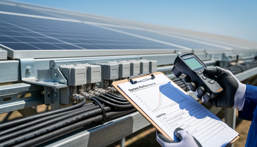
Step 1: Define Project Parameters and Timeline
Start by creating the foundation tab in your spreadsheet with basic project identifiers. Enter the system size in megawatts (MW), this drives all subsequent calculations. A typical utility-scale project ranges from 5 MW to 200+ MW, while commercial installations sit between 0.5 MW and 5 MW.
Document the precise project location, including latitude and longitude coordinates. This determines your solar resource availability and affects degradation assumptions. Specify the technology: monocrystalline PERC modules currently dominate, but bifacial panels are gaining ground for their 5-15% yield boost in suitable terrain.
Set your construction timeline, typically 6-18 months depending on scale. Break this into quarterly milestones if modeling drawdown schedules. Establish the operational period, 25 years remains standard for PPA contracts, though newer projects extend to 30 or 35 years given improved module warranties.
Choose your modeling resolution: monthly periods provide granularity for seasonal revenue variations and debt service coverage, while annual models suffice for high-level feasibility studies. Monthly resolution is essential for construction-phase modeling and tax equity structures.
Step 2: Model Energy Production and Revenue
Energy production forms the core revenue driver of your solar project finance model. Start by inputting hourly or monthly irradiance data from reliable sources like NREL’s NSRDB database or site-specific measurements. Your model should convert this solar resource into AC energy output by applying sequential loss factors.
Calculate the DC energy generation using your system’s rated capacity and the performance ratio that accounts for real-world conditions. Apply derating factors for soiling (typically 2-5% annually depending on location), temperature losses (8-12% in hot climates), inverter efficiency (96-98%), module mismatch (1-2%), and wiring losses (2-3%). Include annual degradation (0.5-0.7% for monocrystalline modules) compounded over the project life.
Revenue modeling requires mapping energy output to contractual structures. For PPA contracts, multiply generation by the contracted rate and any built-in escalators (typically 1-2.5% annually). Merchant revenue depends on forecasted wholesale prices with appropriate discount factors for basis risk. Include capacity payments where applicable and renewable energy credit (REC) values based on state-specific markets.
Account for grid integration costs and any curtailment risk, particularly for projects in congested transmission zones. Build flexibility to toggle between revenue scenarios since lenders will stress-test downside cases where energy prices drop or curtailment increases.
Step 3: Build the Capital Expenditure Schedule
Capital expenditures form the foundation of your solar project’s financial viability, typically representing 60-80% of total project costs. Start by breaking down hardware costs: photovoltaic modules (usually 25-35% of CapEx), inverters (5-10%), mounting structures and tracker systems (8-12%), and electrical balance of system components including transformers, switchgear, and cabling (10-15%).
Soft costs deserve equal attention. Development expenses, land acquisition, interconnection studies, engineering design, and legal fees, often consume 10-20% of budget. Permitting reform initiatives in 2026 are reducing some jurisdictional delays, but budget conservatively for permitting and approval processes.
Structure your construction drawdown schedule to match actual payment milestones: procurement deposits (typically 10-20% upfront), progress payments during installation (monthly or by completion percentage), and retention holdbacks (5-10% until commissioning). Add a 5-10% contingency line item for unforeseen costs, and include financing fees, arrangement fees, commitment fees, and interest during construction, which lenders will capitalize into total project cost. This detailed CapEx schedule directly feeds your debt sizing calculations in subsequent modeling steps.
Step 4: Structure Operating Expenses
Operating expenses form the backbone of your model’s long-term viability and require careful categorization to capture both predictable and variable costs. Start by separating fixed O&M costs, typically $15-25/kW-year for utility-scale projects, from variable expenses tied to production or equipment usage.
Create dedicated line items for insurance (1-2% of capital costs annually), land lease payments (often structured as fixed annual fees or revenue-sharing arrangements), and asset management fees (0.5-1% of revenues). These costs remain relatively stable but still warrant annual escalation at 2-3% to reflect inflation.
Major component replacements demand particular attention. Schedule inverter replacements at years 12-15, using current pricing with 20-30% contingency buffers. Model battery replacements if applicable, typically at 10-year intervals. Don’t overlook transformer maintenance, SCADA system upgrades, and tracker motor replacements for tracking systems.
Apply different escalation rates thoughtfully: insurance may track construction cost indices (3-4%), while labor-intensive O&M might escalate faster (2.5-3.5%) than parts procurement (1.5-2.5%). Link these rates to credible economic forecasts rather than arbitrary assumptions.
Step 5: Configure Financing Structure
Configuring the financing structure transforms your model from a project description into an investment proposition. Begin by establishing your capital stack, the layered arrangement of funding sources that together cover total project costs.
Set up senior debt first, typically comprising 50-70% of total project costs for solar. Input the interest rate (as of 2026, expect 5-8% for investment-grade projects), tenor (usually 15-20 years), and repayment schedule. Most solar projects use sculpted debt, where principal payments are sized to maintain target debt service coverage ratios rather than remaining constant. Create a debt drawdown schedule aligned with your construction expenditure timeline, accounting for commitment fees on undrawn amounts.
Add mezzanine debt if your structure includes it, positioned between senior debt and equity with higher rates (typically 8-12%) reflecting increased risk.
Structure equity contributions next. For tax equity partnerships, model the partnership flip mechanism: tax equity investors contribute capital upfront (often 30-50% of project costs) in exchange for nearly all tax benefits until achieving their target return, then ownership flips predominantly to the sponsor. Input the flip IRR threshold and allocation percentages pre- and post-flip.
Calculate DSCR monthly by dividing cash available for debt service by scheduled debt payments. Target minimum DSCR of 1.20-1.30 during operations, with stricter requirements (1.40+) often mandated in loan covenants. Build covenant tracking directly into your model to flag potential violations before they occur.
Step 6: Calculate Tax Benefits and Incentives
Begin by establishing the tax benefit module as a separate sheet linked to your capital and operating schedules. For 2026 solar projects, model the Investment Tax Credit at its current statutory rate, applying it to eligible basis (qualified capital expenditures excluding land and certain soft costs). Enter the in-service date to trigger the credit in the appropriate tax year.
Create a depreciation schedule using the Modified Accelerated Cost Recovery System. Solar projects qualify for five-year MACRS with bonus depreciation if applicable. Calculate annual depreciation amounts and multiply by the project’s marginal tax rate to determine tax savings. Link these benefits to your cash flow waterfall.
If structuring with tax equity, model the partnership flip mechanics separately. Input the tax equity investor’s contribution percentage and their allocation of tax benefits during the flip period. Calculate when cumulative returns trigger the flip to target allocations, typically when the investor reaches a specified internal rate of return. Track the timing difference between when benefits accrue and when cash distributions occur, this affects project-level returns significantly.
Include state-level incentives as either upfront grants, performance-based payments, or property tax abatements. Model these with appropriate payment schedules and any recapture provisions if project performance thresholds aren’t met.
Step 7: Build Cash Flow Waterfalls and Returns Analysis
Cash flow waterfalls establish the payment hierarchy that protects lenders and attracts investors. Begin by constructing a monthly or annual waterfall that allocates available cash in strict priority: operating expenses and reserves come first, followed by senior debt service, then subordinated debt, tax equity distributions per the partnership agreement, and finally equity returns.
Calculate project-level metrics using these cash flows. Net present value (NPV) discounts all future cash flows to today’s dollars using your weighted average cost of capital. Internal rate of return (IRR) identifies the discount rate where NPV equals zero, lenders typically require minimum project IRRs of 8-10% while equity investors target 12-18%. Don’t confuse project IRR with equity IRR, which measures returns on equity capital alone and runs substantially higher.
Track the equity multiple (total cash returned divided by equity invested) and payback period to give investors additional perspective beyond IRR. These metrics matter because solar ROI presentations require multiple angles to satisfy different investor preferences.
Monitor debt service coverage ratio (DSCR) quarterly, most senior lenders require minimum ratios of 1.20x to 1.35x throughout the loan term. Flag any periods where DSCR falls below covenant thresholds, triggering reserve sweeps or acceleration clauses that fundamentally alter your returns profile.
Adapting Models for Innovative Financing Structures
Standard project finance models provide the foundation, but emerging financing structures demand specific modifications to capture their unique cash flow mechanics and reporting obligations. Each innovative mechanism introduces distinct modeling layers that traditional debt-equity structures don’t address.
Community solar subscription models require tracking individual subscriber accounts within the project cash flow waterfall. Model monthly subscription revenues by cohort, accounting for subscriber acquisition curves, churn rates (typically 8-12% annually), and credit-and-collections cycles. Create separate revenue schedules for anchor subscribers versus residential participants, since anchor tenants often commit to 20-30% of capacity with longer lock-in periods. Your model must calculate the subscriber value-of-solar credit against retail rates, track unsubscribed capacity that sells at wholesale prices, and forecast the net effect on project revenues. Add outputs showing subscription fill rates over time and revenue concentration risk by subscriber size.
Green bonds impose structured reporting requirements that necessitate dedicated tracking modules. Expand your model to isolate eligible green expenditures from total project costs, calculate use-of-proceeds allocations, and generate periodic impact metrics that bond covenants require, tonnes of CO2 avoided, megawatt-hours produced, and fossil fuel displacement figures. Include verification cost line items and schedule semi-annual reporting cycles that bond trustees expect. The model should automatically populate impact dashboards from underlying energy production and emissions factor assumptions.
Blended finance structures combining concessional capital with commercial funding require waterfall modifications showing return priorities across investor classes. Model development finance institution (DFI) tranches with below-market rates or subordinated positions that enhance project returns for commercial lenders. Calculate blended weighted average cost of capital (WACC) across the capital stack, and create sensitivity tables showing how concessional terms improve overall project economics. For structures incorporating zero interest loans or grant elements, separate cash and non-cash subsidies to avoid distorting actual cash-on-cash returns.
Climate fund investments often mandate additionality proofs and gender-lens or local employment metrics. Extend your model to track these non-financial KPIs alongside traditional IRR calculations, creating parallel reporting frameworks that satisfy fund governance requirements while maintaining the project’s core financial logic.

Verification, Stress Testing, and Model Validation
A polished financial model means nothing if the numbers don’t hold up under scrutiny. Before presenting your solar project finance model to investors or lenders, you must verify every calculation, stress-test your assumptions, and prepare documentation that demonstrates the model’s reliability. Lenders routinely reject projects with sloppy models, regardless of the underlying asset quality.
Start with systematic error-checking. Work through each worksheet tab, tracing formulas back to their source cells. Look for hardcoded values where formulas should exist, check that all row and column references increment correctly when copied, and verify that totals match across linked schedules. Pay special attention to time period alignment, revenue in month 37 must correspond to costs and debt service in the same month. Use Excel’s formula auditing tools (trace precedents and dependents) to visualize calculation chains and spot anomalies.
Circular references plague project finance models, especially when modeling tax equity structures or calculating interest on construction debt that depends on cumulative drawdowns. Resolve these by enabling iterative calculation with a maximum of 100 iterations, then verify the circular logic makes mathematical sense. If debt service depends on revenues that depend on production that depends on financing availability, document this relationship clearly and confirm it converges to a stable solution.
Reconciliation checks catch errors formulas alone won’t reveal. Build control totals: sum all cash inflows and verify they equal the sum of all outflows plus ending cash balance. Check that equity contributions plus debt drawdowns equal total capex plus financing fees. Confirm cumulative depreciation plus remaining book value equals original asset cost. These cross-checks expose inconsistencies in model structure.
Before submitting your model, complete these essential verification steps:
- Confirm all external data sources (irradiance, tariffs, interest rates) reflect 2026 market conditions and include supporting documentation
- Verify debt service coverage ratio calculations match lender covenant definitions exactly
- Check that tax benefit timing aligns with partnership flip or sale-leaseback mechanics
- Ensure degradation curves apply consistently across energy production and all dependent revenue streams
- Validate that sensitivity outputs update correctly when input assumptions change
- Test model behavior at extreme values (zero irradiance, 100% cost overruns) to catch divide-by-zero errors
Stress testing reveals project vulnerability. Build downside scenarios that model simultaneous adverse conditions: irradiance 10% below P50, O&M costs running 20% higher than budget, and interest rates 200 basis points above base case. Lenders want to see that debt coverage ratios remain above 1.20x even in these conditions. Run sensitivity tables showing how equity IRR responds to variations in key drivers, module efficiency, capacity factor, PPA price, and construction cost. Two-way sensitivity tables (varying two inputs simultaneously) expose interaction effects that single-variable tests miss.
Third-party validation matters for projects over $50 million. Independent engineers review energy production estimates, technical consultants verify cost assumptions, and tax advisors confirm incentive eligibility. Your model must produce outputs that align with these reports. Prepare a model book (an Excel workbook with assumptions clearly labeled, data sources cited, and calculation methodology explained in dedicated tabs) so validators can audit your work efficiently. Lenders expect summary outputs in standardized formats: sources and uses table, quarterly cash flow waterfalls, and annual DSCR calculations ready for immediate review.
Next Steps: From Model to Financing Close
Completing your project finance model marks the beginning of the financing process, not the end. Your model becomes a living document that evolves through multiple rounds of lender and investor review.
The first deliverable is typically an investment memorandum or financing package. This synthesizes your model into executive-friendly outputs: returns summary, cash flow waterfall diagrams, sensitivity analyses, and key risk metrics. Lenders scrutinize assumptions before they examine outputs, so prepare detailed assumption books that explain every input, its source, and the rationale behind conservative or aggressive positioning. Include comparison benchmarks from similar projects where available.
Technical due diligence follows swiftly. Expect lenders’ independent engineers to challenge degradation rates, O&M cost estimates, and technology risk assessments. You’ll receive detailed question lists requiring model adjustments and re-runs. Maintaining clean, well-documented models with color-coded assumption cells and version control becomes critical. Each iteration should track changes with clear audit trails showing what shifted and why.
Responsive modeling during negotiations often determines financing success. Interest rate movements, changed tax equity pricing, or adjusted PPA terms require immediate model updates. Build flexibility into your structure from the start, dynamic input cells that cascade through calculations without breaking formulas.
Post-financial-close, your model transitions into an operational monitoring tool. Actual performance data replaces projections, triggering covenant compliance checks and investor reporting. Many developers maintain parallel forecast models that update remaining project life based on actual results.
Mastering these advanced techniques requires structured training. Mose Solar’s educational programs, developed in collaboration with leading universities, prepare professionals to navigate the complete project lifecycle from initial modeling through financing close and ongoing asset management, bridging the gap between academic theory and real-world project execution.
Frequently Asked Questions
Building a project finance model for solar energy projects raises practical questions for aspiring PV professionals. Understanding the time investment, required expertise, and data sources helps you approach modeling with realistic expectations and clear next steps.
How long does it take to build a complete solar project finance model?
A basic utility-scale solar finance model typically requires 40-60 hours for someone with intermediate Excel skills and understanding of project finance principles. Complex structures involving tax equity partnerships or multiple revenue streams can extend this to 80-100 hours, while distributed generation portfolios may take less time once you’ve established a template approach.
What level of expertise do I need before attempting to build these models?
You should have strong Excel proficiency (including named ranges, data tables, and complex formulas), basic understanding of renewable energy systems, and familiarity with financial concepts like NPV, IRR, and cash flow waterfalls. Many professionals gain this foundation through university programs partnered with organizations like Mose Solar that integrate financial modeling into their renewable energy curriculum.
What are the key differences between utility-scale and distributed generation modeling?
Utility-scale models focus on single large projects with wholesale power sales and project-level debt, while distributed generation models often aggregate multiple smaller systems, incorporate retail rate structures with demand charges, and may use portfolio-level or corporate financing. Distributed models also require more granular treatment of customer acquisition costs and attrition rates in subscription-based structures.
How do I handle merchant revenue risk in my financial model?
Model merchant exposure by creating multiple price scenarios based on historical wholesale electricity data and forward curves, then calculate probability-weighted returns. Include floor prices using hedge instruments or revenue puts, and stress-test DSCR under downside scenarios to ensure the financing structure can withstand price volatility.
Where can I find reliable input data for irradiance and energy production?
NREL’s National Solar Radiation Database provides validated irradiance data for North American locations, while Meteonorm and SolarGIS offer global coverage. For production estimates, combine satellite data with ground measurements when available, and validate outputs against similar operational projects in your region.
Should I build models from scratch or use templates?
Start with well-structured templates to understand standard modeling conventions and common pitfalls, then customize them for specific project requirements. Building one model completely from scratch helps you grasp the full logic flow, but production work typically involves adapting proven frameworks rather than reinventing the structure for each project.
How often should I update assumptions in an active project model?
Update equipment costs and performance specifications quarterly during development, refresh interest rate and tax assumptions when market conditions shift materially, and recalibrate revenue projections annually or when power purchase agreements are renegotiated. Lock assumptions only after financial close, then maintain a separate tracking model for actual vs. projected performance.
What’s the biggest mistake beginners make in solar finance modeling?
Underestimating the impact of timing assumptions, particularly construction delays, interconnection schedules, and tax credit monetization windows. A six-month delay can fundamentally alter project economics through lost revenue, carrying costs, and potential changes to available incentives, yet many first-time modelers treat these timelines as fixed rather than modeling realistic schedule risk.
These questions reflect the real challenges you’ll encounter as you develop proficiency in solar project finance modeling. The learning curve steepens when you move from textbook examples to actual projects with multiple stakeholders, competing priorities, and real capital at stake.
One frequent concern involves balancing model complexity with usability. While it’s tempting to build increasingly sophisticated models that capture every conceivable variable, lenders and investors value transparency and ease of audit over exhaustive detail. A model that clearly communicates key drivers and assumptions often proves more valuable than one requiring extensive documentation to navigate.
Another practical consideration is version control and collaboration. Solar projects involve multiple parties reviewing and commenting on financial projections. Establishing clear naming conventions, change logs, and a single source of truth prevents the confusion that arises when different stakeholders work from outdated versions with conflicting assumptions.
The transition from academic understanding to professional application requires hands-on practice with real project data. Educational programs offered through university partnerships provide structured pathways to develop these skills under expert guidance, bridging the gap between theoretical knowledge and the messy reality of financing actual solar installations.