When g-formula causal inference models produce implausible results in photovoltaic fault analysis, the most common culprit is positivity violation: your training data lacks sufficient observations across critical combinations of irradiance, temperature, and system states. Before diving into complex debugging, run this quick diagnostic check: plot the empirical density of your treatment variable (panel condition, inverter status, or operational mode) stratified by key confounders. Sparse or zero-density regions signal that your model is extrapolating beyond observed data, generating unreliable counterfactual predictions that can misattribute production losses or recommend unnecessary interventions.
The g-formula offers compelling advantages for predictive maintenance in solar installations because it handles time-varying confounding that standard regression cannot. Yet PV datasets introduce unique challenges: high-frequency sensor noise, seasonal cyclicality, missing data during nighttime hours, and the physical constraints of solar operation create conditions where textbook implementations fail silently.
This troubleshooting guide walks you through systematic diagnosis and correction. We identify the five failure modes most prevalent in photovoltaic applications, from positivity violations and model misspecification to temporal inconsistency and convergence errors. For each, you’ll find concrete diagnostic tests, step-by-step remediation protocols, and validation checks tailored to solar data characteristics. We also address when to abandon the g-formula entirely in favor of alternative causal methods, a critical decision point that can save weeks of fruitless model tuning.
Understanding G-Formula in PV Fault Analysis
The g-formula, formally known as the g-computation formula or standardization formula, estimates what would happen to photovoltaic system performance under different interventions by simulating counterfactual scenarios from observed data. Unlike correlation-based methods that simply identify patterns between variables, the g-formula calculates causal effects by mathematically “intervening” on treatment variables while properly accounting for confounding factors that obscure true cause-and-effect relationships.
In practical terms, traditional PV fault analysis might observe that modules with higher temperatures show more degradation and conclude temperature causes the decline. The g-formula asks a more precise question: if we could set all modules to a specific temperature profile while keeping other conditions representative of real operations, what degradation would we observe? This distinction matters enormously when environmental factors, operating conditions, and failure mechanisms interact in complex ways.
- G-formula
- A statistical method that estimates causal effects by computing standardized outcome distributions under hypothetical interventions, adjusting for measured confounders through marginalization.
- Causal effect
- The difference in outcomes attributable solely to a specific intervention or exposure, isolated from all other contributing factors.
- Counterfactual outcome
- The result that would have occurred under a different treatment or condition than what actually happened, which cannot be directly observed but can be estimated.
- Confounding
- When a third variable influences both the treatment and outcome, creating a spurious association that masks or distorts the true causal relationship.
- Treatment variable
- The exposure, intervention, or condition whose causal effect on an outcome you want to estimate, such as irradiance level or maintenance protocol in PV systems.
- Time-varying covariates
- Variables that change over the observation period and may act as both confounders and intermediate outcomes, such as soiling accumulation or ambient temperature patterns.
The g-formula becomes essential for PV root-cause analysis because photovoltaic systems operate under constantly shifting environmental conditions where simple before-after comparisons fail. When investigating whether micro-cracks cause power loss, you cannot ignore that cracked cells often occur in modules experiencing higher mechanical stress, which itself affects performance. The g-formula disentangles these intertwined relationships by modeling the joint distribution of treatments, confounders, and outcomes, then marginalizing over the confounder distribution to isolate the causal pathway of interest. This approach reveals whether observed associations reflect genuine causal mechanisms or merely correlations driven by shared environmental exposures.
Recognizing Symptoms: When Your G-Formula Implementation Isn’t Working
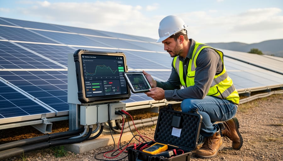
When your g-formula implementation produces suspicious results in photovoltaic fault analysis, recognizing the warning signs early prevents cascading errors in root-cause diagnosis and potentially costly misdiagnoses of system failures.
The first red flag appears when effect estimates swing wildly between iterations. If changing your data aggregation window from hourly to daily measurements produces completely different causal effect magnitudes, say, estimating that inverter curtailment causes a 5% versus 35% reduction in string performance, your g-formula lacks stability. Similarly, adding or removing a single covariate shouldn’t fundamentally alter your conclusions about whether micro-cracking drives power loss.
Implausible effect estimates violate basic physical principles of solar systems. A g-formula suggesting that higher irradiance decreases panel output, or that cooler temperatures worsen thermal stress failures, signals fundamental implementation problems. When your causal inference contradicts established photovoltaic physics, the methodology is flawed regardless of statistical significance.
Several technical symptoms indicate unreliable g-formula implementations:
- Wildly varying causal effect estimates across minor specification changes in model structure
- Effect directions contradicting known physical principles of photovoltaic system operation
- Repeated model convergence failures during iterative parameter estimation procedures
- Extreme predicted probabilities near zero or one that violate realistic operating ranges
Convergence failures manifest as optimization algorithms that never reach stable parameter estimates, often accompanied by warning messages about singular matrices or infinite values. This typically happens when you have insufficient data to estimate complex interaction terms between environmental stressors and degradation pathways.
Contradictory root-cause identification emerges when different subsets of your PV monitoring data point to incompatible failure mechanisms. If January data suggests soiling is the primary fault driver while February data implicates cell degradation for the same underperforming string, your g-formula isn’t capturing the true causal structure, it’s fitting to noise rather than signal.
Watch for extreme propensity scores bunching near the boundaries. If 80% of your observations have estimated treatment probabilities below 0.01 or above 0.99, the positivity assumption breaks down and your causal estimates become unreliable extrapolations rather than data-driven inferences about real PV system behavior.
Root Causes of G-Formula Failures in Photovoltaic Applications

Violation of Positivity Assumption
Photovoltaic monitoring systems often produce data with critical gaps that violate the positivity assumption, a fundamental requirement stating that all individuals must have some probability of receiving each treatment level at every covariate combination. In PV fault analysis, this translates to needing observations across the full range of operating conditions for valid causal inference.
Sparse monitoring creates practical positivity violations. Many solar installations record data at 15-minute intervals but experience rare fault conditions like bypass diode failures or severe hotspots only a handful of times across months. When analyzing irradiance levels above 900 W/m² during winter months at high latitudes, you might have zero observations where certain module temperature ranges coincide with specific fault states. The g-formula cannot estimate causal effects in these empty cells, leading to extreme weights and unstable predictions.
Deterministic system behaviors compound this problem. PV inverters shut down completely below minimum voltage thresholds, a hard constraint that guarantees zero probability of observing certain combinations of string voltage and power output. Similarly, maximum power point tracking algorithms create nearly deterministic relationships between environmental conditions and operating points. When these physical constraints eliminate entire regions of the covariate space, the positivity assumption fails structurally rather than due to limited sample size.
The result is wildly varying causal effect estimates that change dramatically with minor model adjustments, producing unreliable root-cause identification that cannot guide maintenance decisions confidently.
Unmeasured Confounding in Solar Systems
Unmeasured confounding presents one of the most insidious challenges in PV fault analysis because the confounders themselves are often invisible to standard monitoring systems. The g-formula assumes you’ve measured all variables that jointly affect both the treatment (potential fault cause) and outcome (system failure). When critical confounders go unrecorded, your causal estimates drift away from truth, sometimes dramatically.
Micro-shading from nearby structures, vegetation growth, or even soiling accumulation patterns creates localized performance variations that confound the relationship between measured environmental factors and panel degradation. A module might appear to fail due to temperature stress when the true culprit is partial shading your monitoring system never captured. Cell-level degradation mechanisms, solder bond fatigue, encapsulant discoloration, internal corrosion, proceed invisibly until they trigger detectable failures, yet they confound relationships between operating conditions and failure rates.
Soiling doesn’t deposit uniformly across an array. Wind patterns, panel tilt, proximity to pollution sources, and electrostatic effects create heterogeneous soiling that correlates with both environmental exposures and failure modes. When your g-formula specification lacks these spatial soiling patterns, you’ll attribute causality incorrectly to measured variables like humidity or particulate concentration.
The consequence is systematic bias. Your g-formula might suggest that high irradiance causes bypass diode failure when the true mechanism involves unmeasured hotspot formation from manufacturing defects that correlate with high-irradiance installation sites.
Model Misspecification for Complex Failure Pathways
Model misspecification fundamentally undermines g-formula reliability when the assumed mathematical relationships between variables fail to capture the actual physics of PV degradation. Solar systems exhibit inherently non-linear failure pathways that resist simple linear modeling. Temperature effects on power output follow exponential curves, not straight lines. Humidity accelerates corrosion through threshold-dependent mechanisms where mild conditions cause negligible damage but extreme humidity triggers rapid deterioration.
Interaction terms between environmental stressors frequently determine whether faults develop. High temperature alone may not cause hotspots, and localized shading alone may not trigger bypass diode failure, but their simultaneous occurrence creates multiplicative stress that linear models cannot capture. When your g-formula specification omits these critical interaction terms, it attributes effects to individual factors incorrectly.
Time-varying relationships pose additional challenges. Early-life PV module behavior differs markedly from aged module response to identical stressors. A g-formula assuming constant coefficients across system lifetime will produce biased estimates for long-term degradation modes. Cell-level micro-cracks accumulate damage non-linearly, remaining dormant initially before accelerating once critical thresholds are exceeded.
The solution requires incorporating domain knowledge about solar physics directly into model specifications. Include polynomial terms for known non-linear relationships, explicitly model interactions between correlated stressors, and allow time-varying coefficients when analyzing degradation patterns across extended operational periods.
Insufficient Sample Size for Rare Fault Modes
Rare fault modes in photovoltaic systems present a statistical challenge that directly undermines g-formula reliability. When critical failures like bypass diode malfunctions or localized hotspots occur infrequently, perhaps affecting only 2-3% of modules in your dataset, the algorithm struggles to learn meaningful causal relationships from such limited examples.
This sparsity creates unstable parameter estimates in the g-formula’s outcome models. With few observed instances of a fault type, the algorithm cannot reliably distinguish true causal effects from random noise. You’ll see exaggerated effect sizes and confidence intervals that span impractically wide ranges, rendering predictions nearly useless for operational decisions.
The problem compounds when analyzing interaction effects. If you’re investigating how temperature stress interacts with manufacturing batch to cause hotspots, sparse cells emerge rapidly. A dataset with 1,000 modules might yield only 15 hotspot cases, spread across multiple temperature ranges and dozens of batches. Each cell in your cross-tabulation contains too few observations for stable estimation.
Consequences include failed model convergence, wildly inconsistent results across bootstrap iterations, and causal effect estimates that flip sign unpredictably when you add or remove single data points.
Step-by-Step Fix: Implementing Robust G-Formula Analysis for PV Faults
Step 1: Verify and Strengthen Data Quality
Data quality forms the foundation of reliable g-formula causal inference in PV fault analysis. Begin by auditing your monitoring dataset for completeness, check timestamp continuity, identify gaps in sensor readings, and calculate the percentage of missing values for each variable. Incomplete data creates sparse cells that destabilize causal effect estimation.
Validate sensor calibration by comparing readings against manufacturer specifications and cross-checking correlated measurements (irradiance sensors versus expected current output). Miscalibrated sensors introduce systematic bias that propagates through the entire g-formula calculation, producing incorrect root-cause conclusions.
Aggregate data to an appropriate temporal resolution that balances statistical power with physical relevance. Hourly or daily averages often work better than raw minute-level data for fault analysis, reducing noise while preserving genuine degradation signals. This aggregation enables real-time optimization of monitoring protocols.
Handle missing values using domain-appropriate methods, forward-fill for slowly-changing environmental variables, but avoid imputation for fault indicators where missingness itself may signal sensor failure. Document all preprocessing decisions to ensure reproducibility and facilitate sensitivity analysis of data quality assumptions.
Step 2: Check and Address Positivity Violations
Positivity violations occur when certain combinations of environmental conditions or system states never appear in your PV dataset, creating empty cells that destabilize causal estimates. Start by cross-tabulating treatment levels (fault presence/absence) against key covariates like irradiance bins, temperature ranges, and system age categories. Look for combinations with zero or very few observations, these signal positivity problems.
Calculate propensity scores to visualize overlap. Plot the distribution of estimated probabilities for developing faults across different covariate patterns. If you see propensity scores bunched at 0 or 1, your data lacks sufficient overlap between faulty and healthy systems under similar conditions. This commonly happens with extreme operating scenarios, very high temperatures combined with specific shading patterns, for instance.
Address violations by trimming the tails: exclude observations with propensity scores below 0.05 or above 0.95, restricting inference to regions where both fault states occur. Alternatively, combine sparse covariate categories, merge adjacent irradiance bins or broader temperature ranges, to achieve adequate sample sizes in each cell. This trades some precision for stability, but produces more reliable causal estimates than forcing the g-formula through impossible extrapolations in PV operating space.
Step 3: Refine Confounding Control Strategy
Start by mapping your photovoltaic failure pathways in a directed acyclic graph. Draw nodes for the fault outcome you’re analyzing, the suspected root causes, and all intermediate variables. Connect these with arrows showing causal direction based on solar physics principles: incident irradiance affects module temperature, temperature influences power conversion efficiency, efficiency impacts thermal stress, stress contributes to solder joint fatigue. This visualization reveals which variables confound your causal estimates.
Identify the minimal sufficient adjustment set from your DAG, the smallest collection of variables that blocks all backdoor paths between treatment and outcome. You don’t need to control for every measured variable; controlling for colliders or mediators actually introduces bias. For PV analysis, this typically includes ambient conditions, system age, and inverter operating parameters, but not variables that lie on the causal pathway itself.
Incorporate proxy measurements when direct confounders are unavailable. Can’t measure cell-level soiling? Use rainfall frequency and site particulate matter readings as proxies. Missing micro-shading data? Include nearby vegetation indices from satellite imagery. These proxies won’t eliminate confounding entirely, but they reduce bias substantially compared to ignoring unmeasured factors. Document which confounders remain unmeasured for your sensitivity analysis in Step 5.
Step 4: Improve Outcome and Treatment Models
The outcome and treatment models form the computational core of your g-formula implementation, and their quality determines whether you’ll get reliable causal estimates. Replace simple linear regression with machine learning models like random forests or gradient boosting that capture the non-linear relationships inherent in PV system failures. These methods handle interactions between temperature, irradiance and degradation without requiring you to manually specify every possible combination.
Include physically meaningful interactions based on solar engineering principles. Temperature affects semiconductor performance exponentially, not linearly. Shading impacts are multiplicative with bypass diode states. Soiling accumulation depends on both rainfall frequency and panel tilt angle. Build these known physics relationships into your feature engineering rather than hoping the algorithm discovers them.
Validate your model specifications using residual diagnostics tailored to PV data patterns. Plot residuals against time of day to catch circadian effects you missed. Check residuals across irradiance bins to identify non-linearities in light response. Examine spatial patterns in residual maps to detect unmodeled geographic confounders like micro-climate zones. If residuals show structure, your functional form is wrong and your causal estimates will be biased.
Step 5: Validate Results and Conduct Sensitivity Analysis
After implementing your refined g-formula model, validation separates credible causal insights from statistical artifacts. Start by checking whether your estimated effects align with solar physics fundamentals, if the analysis suggests that higher irradiance reduces output, something has gone wrong. Compare magnitudes against published degradation rates and failure mechanisms documented in peer-reviewed photovoltaic literature.
Perform sensitivity analyses to quantify how unmeasured confounders might bias your conclusions. Use E-value calculations to determine the minimum strength of unmeasured confounding needed to nullify your findings. For PV fault analysis, test scenarios where unobserved micro-shading or cell-level defects could influence both treatment assignment and failure outcomes. If plausible unmeasured factors could easily explain away your causal estimates, interpret results cautiously.
When available, validate g-formula predictions against controlled experiments, A/B tests on maintenance interventions, or quasi-experimental designs like regression discontinuity around warranty replacement thresholds. Cross-reference your root-cause attributions with findings from predicting failures models or digital twins that simulate fault propagation under different scenarios.
Quantify uncertainty through bootstrapping to generate confidence intervals for your causal effect estimates. Report both point estimates and credible ranges, acknowledging that observational PV data rarely supports the precision of randomized trials. Document all validation checks and sensitivity analyses transparently, so stakeholders understand the robustness and limitations of your causal inferences before making operational decisions.
Preventing Future G-Formula Implementation Problems
Establish a sustainable causal inference framework by building quality controls into your workflow from the outset rather than troubleshooting failures after they emerge. Start with prospective data collection planning: define the specific causal questions you need to answer before deploying monitoring infrastructure, then design sensor networks to capture relevant confounders including micro-climate variables, electrical loading patterns, and module-level degradation indicators. This upfront investment prevents the sparse data and unmeasured confounding that destabilize g-formula implementations in photovoltaic contexts.
Develop explicit algorithm selection criteria based on your data characteristics and inferential goals. For frequent, well-documented failure modes with abundant data, parametric g-formula implementations may suffice. When analyzing rare faults or complex degradation pathways, opt for doubly robust methods that combine g-formula with inverse probability weighting to maintain validity even when sub-models are imperfectly specified. Document these selection rules so analysis choices remain consistent and defensible across projects.
Institute ongoing validation protocols that systematically stress-test your causal inference pipeline. Schedule quarterly reviews where you compare g-formula effect estimates against newly available experimental data, manufacturer field reports, or independent validation datasets from similar PV installations. When estimates diverge from domain expectations, treat this as an early warning signal rather than waiting for complete failure. Create automated checks that flag positivity violations, extreme propensity scores, or insufficient effective sample sizes before they propagate into unreliable causal conclusions.
Maintain a living library of directed acyclic graphs for common PV failure pathways, updating these causal diagrams as new research emerges about degradation mechanisms and environmental stressors. This shared knowledge base ensures that new team members and projects benefit from accumulated domain wisdom rather than rediscovering confounding structures through trial and error. Combined with robust data infrastructure, these practices help prevent system failures in both your photovoltaic installations and the analytical frameworks that diagnose them.
How to Prevent It Next Time

Establish prevention protocols before your next PV fault analysis project begins. Design monitoring systems with g-formula requirements in mind, deploy sensors that capture confounding environmental variables like irradiance variability, temperature gradients, and soiling accumulation patterns from day one rather than retrofitting data collection later.
Create standardized data quality checkpoints in your workflow. Schedule quarterly reviews of sensor calibration, missing data patterns, and covariate balance across treatment groups. These regular audits catch positivity violations and sparse data regions before they compromise causal estimates.
Build a validation library specific to your PV systems. Document known causal relationships from controlled experiments or manufacturer specifications, then use these as benchmarks to sanity-check g-formula outputs. When estimates contradict established physics, investigate model specification rather than accepting implausible results.
Maintain living DAGs that evolve with your understanding of failure mechanisms. Update these causal diagrams as you discover new degradation pathways or environmental interactions, ensuring your confounding control strategy stays current with emerging knowledge about photovoltaic system behavior.
Invest in ongoing training for your analytical team. As causal inference methods advance and PV technologies change, continuous education prevents outdated implementation practices from introducing subtle errors.
At-a-Glance Details
| G-Formula Component | PV-Specific Challenge | Quick Diagnostic | First Action |
|---|---|---|---|
| Positivity | Sparse data in extreme weather conditions | Check propensity score distribution for values near 0 or 1 | Restrict analysis to common operating ranges |
| Confounding Control | Unmeasured micro-shading and soiling | Compare effect estimates with and without environmental proxies | Add spatial and temporal covariates |
| Model Specification | Non-linear degradation patterns | Plot residuals against irradiance and temperature | Include polynomial terms and interactions |
| Sample Size | Rare failure modes in fault data | Count events per covariate stratum | Pool similar failure types or extend monitoring period |
This diagnostic matrix provides a rapid reference when your g-formula analysis produces questionable results. Each row targets a distinct assumption that frequently breaks in photovoltaic applications, helping you prioritize troubleshooting efforts based on the specific patterns you observe in your fault analysis workflow.
Frequently Asked Questions
Practitioners implementing g-formula causal inference for photovoltaic fault diagnosis often encounter similar challenges and questions. Understanding when and how to apply this method effectively can save considerable troubleshooting time and improve analytical reliability.
When should I use g-formula instead of other causal inference methods for PV fault analysis?
Choose g-formula when you need to estimate effects of sustained interventions or multiple treatment strategies in PV systems, particularly when analyzing complex failure pathways with time-varying confounders like environmental conditions. For simpler scenarios with point treatments and no time-varying confounding, propensity score methods or instrumental variables may be more straightforward.
What is the minimum sample size needed for reliable g-formula estimates in photovoltaic applications?
There is no universal threshold, but you generally need enough observations in each treatment-covariate combination to estimate stable outcome models, typically hundreds of failure events for rare fault modes and thousands of system-months for degradation analyses. Sparse cells with fewer than 10-20 observations per covariate pattern often produce unreliable estimates.
How do I handle time-varying confounders like irradiance and temperature in solar degradation studies?
Use sequential g-formula (also called g-computation formula for time-varying treatments) to properly account for confounders that change over time and are affected by prior treatments. This approach models the joint evolution of treatments, confounders, and outcomes across multiple time points, which is essential for accurate degradation pathway analysis.
What are my alternatives if g-formula assumptions cannot be satisfied with my PV data?
Consider doubly-robust methods combining g-formula with inverse probability weighting for added protection against model misspecification, use sensitivity analyses to quantify potential bias from unmeasured confounding, or shift to alternative causal frameworks like regression discontinuity or difference-in-differences if your PV system installation or operational changes create appropriate quasi-experimental designs.
Beyond these foundational questions, professionals should recognize that g-formula implementation requires iterative refinement. Initial attempts may reveal data quality issues or assumption violations that necessitate returning to earlier diagnostic steps. This is normal in causal inference workflows, particularly when adapting statistical methods developed for biomedical research to the unique characteristics of photovoltaic systems.
The interaction between statistical assumptions and physical reality in solar systems creates unique challenges. Environmental confounders exhibit strong temporal autocorrelation, degradation mechanisms operate on multiple timescales simultaneously, and measurement limitations mean some critical variables remain unmeasured. Successfully navigating these challenges requires both statistical sophistication and deep understanding of photovoltaic physics, making collaboration between data scientists and solar engineers particularly valuable for robust causal inference implementations.
Key Takeaways for PV Professionals
Successfully applying g-formula causal inference to photovoltaic fault diagnosis demands more than statistical proficiency. You need deep integration of causal reasoning with solar engineering expertise. The method’s power lies in its ability to separate true causal effects from spurious correlations, but only when its assumptions align with your PV data characteristics.
Start every analysis by constructing a directed acyclic graph that maps physical degradation pathways and environmental interactions in your specific solar installation. This DAG serves as your roadmap for identifying confounders and preventing bias. Don’t skip this step, attempting to implement g-formula without explicit causal structure inevitably leads to unreliable root-cause identification.
Recognize that PV monitoring data often violates the positivity assumption. Arrays rarely experience certain combinations of environmental stressors simultaneously, creating sparse regions where causal effects cannot be estimated. Address this through propensity trimming or restrict your causal claims to well-supported operating ranges rather than forcing unstable extrapolation.
Machine learning methods like random forests substantially improve g-formula performance for PV applications compared to simple linear models. Solar degradation involves complex interactions between temperature, irradiance, humidity and system age that flexible algorithms capture naturally. However, always validate that your models respect known physical constraints and produce sensible intermediate predictions.
Never treat g-formula as a black box. Conduct rigorous sensitivity analyses quantifying how unmeasured confounders could shift your conclusions. Compare causal estimates against domain expectations and, when possible, experimental validation data. The goal is defendable causal inference that advances practical fault mitigation, not just statistically significant results.
When sample sizes prove insufficient for rare fault modes or deterministic system behaviors create fundamental positivity violations, acknowledge these limitations explicitly. Alternative approaches like instrumental variables or natural experiments may provide more reliable causal insights for specific PV failure mechanisms.
Successfully implementing g-formula causal inference in photovoltaic fault analysis delivers transformative diagnostic capabilities that move beyond correlation to identify true root causes of system failures. However, this power comes with responsibility: the method demands rigorous attention to its core assumptions, positivity, conditional exchangeability, and consistency, each of which requires domain-specific adaptations when working with solar data.
The journey from implementation failure to reliable causal insights follows a clear path: systematic data quality verification, careful assessment of assumption violations, flexible modeling that respects PV physics, and thorough validation against engineering expectations. When you address positivity violations through appropriate sample restrictions, control confounding with physically informed DAGs, and specify models that capture non-linear degradation mechanisms, the g-formula reveals causal relationships that traditional analytics miss entirely.
The solar industry needs professionals who understand both statistical methodology and photovoltaic engineering. Mose Solar collaborates with leading universities to develop educational programs that equip the next generation of PV professionals with these dual competencies, including training in Causal AI applications for renewable energy systems. This intersection of disciplines represents where photovoltaic diagnostics is headed, combining rigorous causal inference with deep solar domain expertise to build more reliable, efficient renewable energy infrastructure.